HOME

SCHEDULE

RESOURCES

GLOSSARY

ASSIGNMENTS

DOMAIN TESTING:

This unit gives an indepth overview of domain testing and its implementation.

At the end of this unit, the student will be able to:

• Understand the concept of domain testing.
• Understand the importance and limitations of domain testing.
• Differentiate ugly and nice domains.
• Know the properties of ugly and nice domains.
• Learn the domain testing strategy for different dimension domains.
• Identify the problems due to the incompatibility of domains and ranges in interface testing.

---

DOMAINS AND PATHS:

---

• INTRODUCTION:
  • Domain:In mathematics, domain is a set of possible values of an independant variable or the variables of a function.
  • Programs as input data classifiers: domain testing attempts to determine whether the classification is or is not correct.
  • Domain testing can be based on specifications or equivalent implementation information.
  • If domain testing is based on specifications, it is a functional test technique.
  • If domain testing is based implementation details, it is a structural test technique.
  • For example, you're doing domain testing when you check extreme values of an input variable.

  All inputs to a program can be considered as if they are numbers. For example, a character string can be treated as a number by concatenating bits and looking at them as if they were a binary integer. This is the view in domain testing, which is why this strategy has a mathematical flavor.

• THE MODEL: The following figure is a schematic representation of domain testing.
  
  
  
  

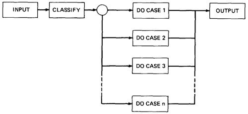
  Figure 4.1: Schematic Representation of Domain Testing.

  • Before doing whatever it does, a routine must classify the input and set it moving on the right path.
  • An invalid input (e.g., value too big) is just a special processing case called 'reject'.
  • The input then passses to a hypothetical subroutine rather than on calculations.
  • In domain testing, we focus on the classification aspect of the routine rather than on the calculations.
  • Structural knowledge is not needed for this model - only a consistent, complete specification of input values for each case.
  • We can infer that for each case there must be atleast one path to process that case.
• A DOMAIN IS A SET:
  • An input domain is a set.
  • If the source language supports set definitions (E.g. PASCAL set types and C enumerated types) less testing is needed because the compiler does much of it for us.
  • Domain testing does not work well with arbitrary discrete sets of data objects.
  • Domain for a loop-free program corresponds to a set of numbers defined over the input vector.
• DOMAINS, PATHS AND PREDICATES:
  • In domain testing, predicates are assumed to be interpreted in terms of input vector variables.
  • If domain testing is applied to structure, then predicate interpretation must be based on actual paths through the routine - that is, based on the implementation control flowgraph.
  • Conversely, if domain testing is applied to specifications, interpretation is based on a specified data flowgraph for the routine; but usually, as is the nature of specifications, no interpretation is needed because the domains are specified directly.
  • For every domain, there is at least one path through the routine.
  • There may be more than one path if the domain consists of disconnected parts or if the domain is defined by the union of two or more domains.
  • Domains are defined their boundaries. Domain boundaries are also where most domain bugs occur.
  • For every boundary there is at least one predicate that specifies what numbers belong to the domain and what numbers don't.
    
    For example, in the statement IF x>0 THEN ALPHA ELSE BETA we know that numbers greater than zero belong to ALPHA processing domain(s) while zero and smaller numbers belong to BETA domain(s).
    
    
  • A domain may have one or more boundaries - no matter how many variables define it.
    
    For example, if the predicate is x2 + y2 < 16, the domain is the inside of a circle of radius 4 about the origin. Similarly, we could define a spherical domain with one boundary but in three variables.
    
    
  • Domains are usually defined by many boundary segments and therefore by many predicates. i.e. the set of interpreted predicates traversed on that path (i.e., the path's predicate expression) defines the domain's boundaries.
• A DOMAIN CLOSURE:
  • A domain boundary is closed with respect to a domain if the points on the boundary belong to the domain.
  • If the boundary points belong to some other domain, the boundary is said to be open.
  • Figure 4.2 shows three situations for a one-dimensional domain - i.e., a domain defined over one input variable; call it x
  • The importance of domain closure is that incorrect closure bugs are frequent domain bugs. For example, x >= 0 when x > 0 was intended.
  
  
  
  
  

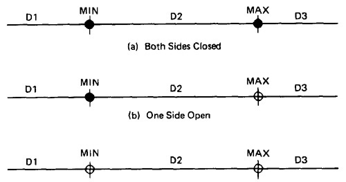
  Figure 4.2: Open and Closed Domains.

• DOMAIN DIMENSIONALITY:
  • Every input variable adds one dimension to the domain.
  • One variable defines domains on a number line.
  • Two variables define planar domains.
  • Three variables define solid domains.
  • Every new predicate slices through previously defined domains and cuts them in half.
  • Every boundary slices through the input vector space with a dimensionality which is less than the dimensionality of the space.
  • Thus, planes are cut by lines and points, volumes by planes, lines and points and n-spaces by hyperplanes.
• BUG ASSUMPTION:
  • The bug assumption for the domain testing is that processing is okay but the domain definition is wrong.
  • An incorrectly implemented domain means that boundaries are wrong, which may in turn mean that control flow predicates are wrong.
  • Many different bugs can result in domain errors. Some of them are:
    Domain Errors:
    • Double Zero Representation :In computers or Languages that have a distinct positive and negative zero, boundary errors for negative zero are common.
    • Floating point zero check:A floating point number can equal zero only if the previous definition of that number set it to zero or if it is subtracted from it self or multiplied by zero. So the floating point zero check to be done against a epsilon value.
    • Contradictory domains:An implemented domain can never be ambiguous or contradictory, but a specified domain can. A contradictory domain specification means that at least two supposedly distinct domains overlap.
    • Ambiguous domains:Ambiguous domains means that union of the domains is incomplete. That is there are missing domains or holes in the specified domains. Not specifying what happens to points on the domain boundary is a common ambiguity.
    • Overspecified Domains:he domain can be overloaded with so many conditions that the result is a null domain. Another way to put it is to say that the domain's path is unachievable.
    • Boundary Errors:Errors caused in and around the boundary of a domain. Example, boundary closure bug, shifted, tilted, missing, extra boundary.
    • Closure Reversal:A common bug. The predicate is defined in terms of >=. The programmer chooses to implement the logical complement and incorrectly uses <= for the new predicate; i.e., x >= 0 is incorrectly negated as x <= 0, thereby shifting boundary values to adjacent domains.
    • Faulty Logic:Compound predicates (especially) are subject to faulty logic transformations and improper simplification. If the predicates define domain boundaries, all kinds of domain bugs can result from faulty logic manipulations.
• RESTRICTIONS TO DOMAIN TESTING:Domain testing has restrictions, as do other testing techniques. Some of them include:
  • Co-incidental Correctness:Domain testing isn't good at finding bugs for which the outcome is correct for the wrong reasons. If we're plagued by coincidental correctness we may misjudge an incorrect boundary. Note that this implies weakness for domain testing when dealing with routines that have binary outcomes (i.e., TRUE/FALSE)
  • Representative Outcome:Domain testing is an example of partition testing. Partition-testing strategies divide the program's input space into domains such that all inputs within a domain are equivalent (not equal, but equivalent) in the sense that any input represents all inputs in that domain. If the selected input is shown to be correct by a test, then processing is presumed correct, and therefore all inputs within that domain are expected (perhaps unjustifiably) to be correct. Most test techniques, functional or structural, fall under partition testing and therefore make this representative outcome assumption. For example, x² and 2^x are equal for x = 2, but the functions are different. The functional differences between adjacent domains are usually simple, such as x + 7 versus x + 9, rather than x² versus 2^x.
  • Simple Domain Boundaries and Compound Predicates:Compound predicates in which each part of the predicate specifies a different boundary are not a problem: for example, x >= 0 AND x < 17, just specifies two domain boundaries by one compound predicate. As an example of a compound predicate that specifies one boundary, consider: x = 0 AND y >= 7 AND y <= 14. This predicate specifies one boundary equation (x = 0) but alternates closure, putting it in one or the other domain depending on whether y < 7 or y > 14. Treat compound predicates with respect because they’re more complicated than they seem.
  • Functional Homogeneity of Bugs:Whatever the bug is, it will not change the functional form of the boundary predicate. For example, if the predicate is ax >= b, the bug will be in the value of a or b but it will not change the predicate to ax >= b, say.
  • Linear Vector Space:Most papers on domain testing, assume linear boundaries - not a bad assumption because in practice most boundary predicates are linear.
  • Loop Free Software:Loops are problematic for domain testing. The trouble with loops is that each iteration can result in a different predicate expression (after interpretation), which means a possible domain boundary change.

---

NICE AND UGLY DOMAINS:

---

• NICE DOMAINS:
  • Where does these domains come from?
    Domains are and will be defined by an imperfect iterative process aimed at achieving (user, buyer, voter) satisfaction.
  • Implemented domains can't be incomplete or inconsistent. Every input will be processed (rejection is a process), possibly forever. Inconsistent domains will be made consistent.
  • Conversely, specified domains can be incomplete and/or inconsistent. Incomplete in this context means that there are input vectors for which no path is specified, and inconsistent means that there are at least two contradictory specifications over the same segment of the input space.
  • Some important properties of nice domains are: Linear, Complete, Systematic, Orthogonal, Consistently closed, Convex and Simply connected.
  • To the extent that domains have these properties domain testing is easy as testing gets.
  • The bug frequency is lesser for nice domain than for ugly domains.
  
  
  
  
  

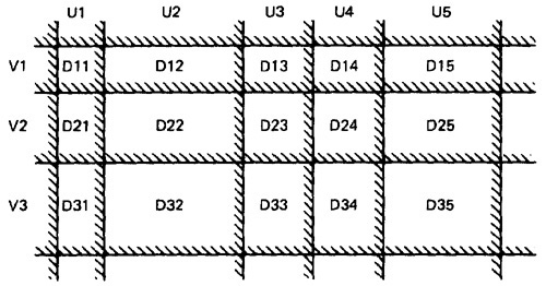
  Figure 4.3: Nice Two-Dimensional Domains.

• LINEAR AND NON LINEAR BOUNDARIES:
  • Nice domain boundaries are defined by linear inequalities or equations.
  • The impact on testing stems from the fact that it takes only two points to determine a straight line and three points to determine a plane and in general n+1 points to determine a n-dimensional hyper plane.
  • In practice more than 99.99% of all boundary predicates are either linear or can be linearized by simple variable transformations.
• COMPLETE BOUNDARIES:
  • Nice domain boundaries are complete in that they span the number space from plus to minus infinity in all dimensions.
  • Figure 4.4 shows some incomplete boundaries. Boundaries A and E have gaps.
  • Such boundaries can come about because the path that hypothetically corresponds to them is unachievable, because inputs are constrained in such a way that such values can't exist, because of compound predicates that define a single boundary, or because redundant predicates convert such boundary values into a null set.
  • The advantage of complete boundaries is that one set of tests is needed to confirm the boundary no matter how many domains it bounds.
  • If the boundary is chopped up and has holes in it, then every segment of that boundary must be tested for every domain it bounds.
  
  
  
  
  

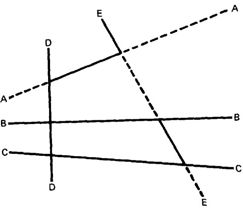
  Figure 4.4: Incomplete Domain Boundaries.

• SYSTEMATIC BOUNDARIES:
  • Systematic boundary means that boundary inequalities related by a simple function such as a constant.
  • In Figure 4.3 for example, the domain boundaries for u and v differ only by a constant. We want relations such as
    
    
    
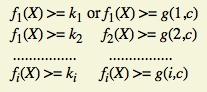
    where f_i is an arbitrary linear function, X is the input vector, k_i and c are constants, and g(i,c) is a decent function over i and c that yields a constant, such as k + ic.
  • The first example is a set of parallel lines, and the second example is a set of systematically (e.g., equally) spaced parallel lines (such as the spokes of a wheel, if equally spaced in angles, systematic).
  • If the boundaries are systematic and if you have one tied down and generate tests for it, the tests for the rest of the boundaries in that set can be automatically generated.
• ORTHOGONAL BOUNDARIES:
  • Two boundary sets U and V (See Figure 4.3) are said to be orthogonal if every inequality in V is perpendicular to every inequality in U.
  • If two boundary sets are orthogonal, then they can be tested independently
  • In Figure 4.3 we have six boundaries in U and four in V. We can confirm the boundary properties in a number of tests proportional to 6 + 4 = 10 (O(n)). If we tilt the boundaries to get Figure 4.5, we must now test the intersections. We've gone from a linear number of cases to a quadratic: from O(n) to O(n²).
    
    
    
    

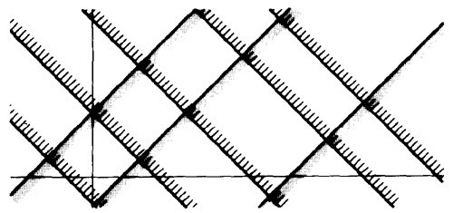
    Figure 4.5: Tilted Boundaries.

    ---

    
    
    
    
    

    Figure 4.6: Linear, Non-orthogonal Domain Boundaries.

  • Actually, there are two different but related orthogonality conditions. Sets of boundaries can be orthogonal to one another but not orthogonal to the coordinate axes (condition 1), or boundaries can be orthogonal to the coordinate axes (condition 2).
• CLOSURE CONSISTENCY:
  • Figure 4.6 shows another desirable domain property: boundary closures are consistent and systematic.
  • The shaded areas on the boundary denote that the boundary belongs to the domain in which the shading lies - e.g., the boundary lines belong to the domains on the right.
  • Consistent closure means that there is a simple pattern to the closures - for example, using the same relational operator for all boundaries of a set of parallel boundaries.
• CONVEX:
  • A geometric figure (in any number of dimensions) is convex if you can take two arbitrary points on any two different boundaries, join them by a line and all points on that line lie within the figure.
  • Nice domains are convex; dirty domains aren't.
  • You can smell a suspected concavity when you see phrases such as: ". . . except if . . .," "However . . .," ". . . but not. . . ." In programming, it's often the buts in the specification that kill you.
• SIMPLY CONNECTED:
  • Nice domains are simply connected; that is, they are in one piece rather than pieces all over the place interspersed with other domains.
  • Simple connectivity is a weaker requirement than convexity; if a domain is convex it is simply connected, but not vice versa.
  • Consider domain boundaries defined by a compound predicate of the (boolean) form ABC. Say that the input space is divided into two domains, one defined by ABC and, therefore, the other defined by its negation .
  • For example, suppose we define valid numbers as those lying between 10 and 17 inclusive. The invalid numbers are the disconnected domain consisting of numbers less than 10 and greater than 17.
  • Simple connectivity, especially for default cases, may be impossible.

  ---

• UGLY DOMAINS:
  • Some domains are born ugly and some are uglified by bad specifications.
  • Every simplification of ugly domains by programmers can be either good or bad.
  • Programmers in search of nice solutions will "simplify" essential complexity out of existence. Testers in search of brilliant insights will be blind to essential complexity and therefore miss important cases.
  • If the ugliness results from bad specifications and the programmer's simplification is harmless, then the programmer has made ugly good.
  • But if the domain's complexity is essential (e.g., the income tax code), such "simplifications" constitute bugs.
  • Nonlinear boundaries are so rare in ordinary programming that there's no information on how programmers might "correct" such boundaries if they're essential.
• AMBIGUITIES AND CONTRADICTIONS:
  • Domain ambiguities are holes in the input space.
  • The holes may lie with in the domains or in cracks between domains.
    
    
    
    

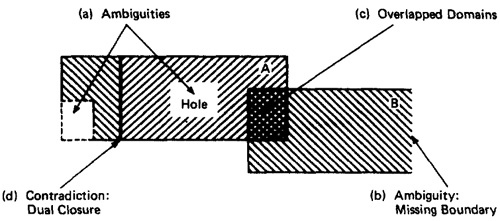
    Figure 4.7: Domain Ambiguities and Contradictions.

  • Two kinds of contradictions are possible: overlapped domain specifications and overlapped closure specifications
  • Figure 4.7c shows overlapped domains and Figure 4.7d shows dual closure assignment.
• SIMPLIFYING THE TOPOLOGY:
  • The programmer's and tester's reaction to complex domains is the same - simplify
  • There are three generic cases: concavities, holes and disconnected pieces.
  • Programmers introduce bugs and testers misdesign test cases by: smoothing out concavities (Figure 4.8a), filling in holes (Figure 4.8b), and joining disconnected pieces (Figure 4.8c).
    
    
    
    

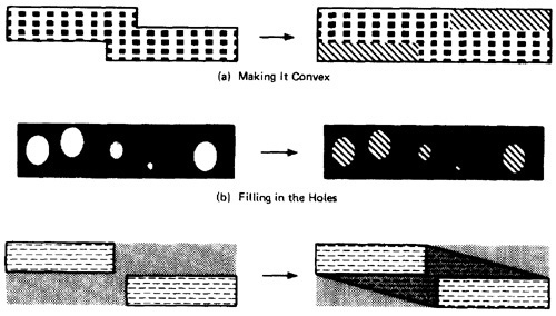
    Figure 4.8: Simplifying the topology.

• RECTIFYING BOUNDARY CLOSURES:
  • If domain boundaries are parallel but have closures that go every which way (left, right, left, . . .) the natural reaction is to make closures go the same way (see Figure 4.9).
    
    
    
    

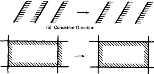
    Figure 4.9: Forcing Closure Consistency.

---

DOMAIN TESTING:

---

• DOMAIN TESTING STRATEGY: The domain-testing strategy is simple, although possibly tedious (slow).
  1. Domains are defined by their boundaries; therefore, domain testing concentrates test points on or near boundaries.
  2. Classify what can go wrong with boundaries, then define a test strategy for each case. Pick enough points to test for all recognized kinds of boundary errors.
  3. Because every boundary serves at least two different domains, test points used to check one domain can also be used to check adjacent domains. Remove redundant test points.
  4. Run the tests and by posttest analysis (the tedious part) determine if any boundaries are faulty and if so, how.
  5. Run enough tests to verify every boundary of every domain.
• DOMAIN BUGS AND HOW TO TEST FOR THEM:
  • An interior point (Figure 4.10) is a point in the domain such that all points within an arbitrarily small distance (called an epsilon neighborhood) are also in the domain.
  • A boundary point is one such that within an epsilon neighborhood there are points both in the domain and not in the domain.
  • An extreme point is a point that does not lie between any two other arbitrary but distinct points of a (convex) domain.
    
    
    
    

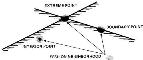
    Figure 4.10: Interior, Boundary and Extreme points.

  • An on point is a point on the boundary.
  • If the domain boundary is closed, an off point is a point near the boundary but in the adjacent domain.
  • If the boundary is open, an off point is a point near the boundary but in the domain being tested; see Figure 4.11. You can remember this by the acronym COOOOI: Closed Off Outside, Open Off Inside.
    
    
    
    

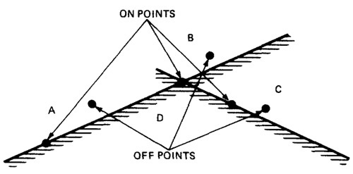
    Figure 4.11: On points and Off points.

  • Figure 4.12 shows generic domain bugs: closure bug, shifted boundaries, tilted boundaries, extra boundary, missing boundary.
    
    
    
    

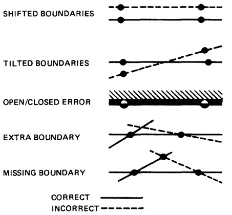
    Figure 4.12: Generic Domain Bugs.

• TESTING ONE DIMENSIONAL DOMAINS:
  • Figure 4.13 shows possible domain bugs for a one-dimensional open domain boundary.
  • The closure can be wrong (i.e., assigned to the wrong domain) or the boundary (a point in this case) can be shifted one way or the other, we can be missing a boundary, or we can have an extra boundary.
    
    
    
    

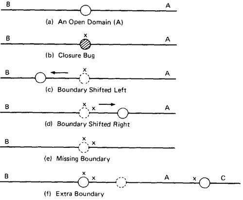
    Figure 4.13: One Dimensional Domain Bugs, Open Boundaries.

  • In Figure 4.13a we assumed that the boundary was to be open for A. The bug we're looking for is a closure error, which converts > to >= or < to <= (Figure 4.13b). One test (marked x) on the boundary point detects this bug because processing for that point will go to domain A rather than B.
  • In Figure 4.13c we've suffered a boundary shift to the left. The test point we used for closure detects this bug because the bug forces the point from the B domain, where it should be, to A processing. Note that we can't distinguish between a shift and a closure error, but we do know that we have a bug.
  • Figure 4.13d shows a shift the other way. The on point doesn't tell us anything because the boundary shift doesn't change the fact that the test point will be processed in B. To detect this shift we need a point close to the boundary but within A. The boundary is open, therefore by definition, the off point is in A (Open Off Inside).
  • The same open off point also suffices to detect a missing boundary because what should have been processed in A is now processed in B.
  • To detect an extra boundary we have to look at two domain boundaries. In this context an extra boundary means that A has been split in two. The two off points that we selected before (one for each boundary) does the job. If point C had been a closed boundary, the on test point at C would do it.
  • For closed domains look at Figure 4.14. As for the open boundary, a test point on the boundary detects the closure bug. The rest of the cases are similar to the open boundary, except now the strategy requires off points just outside the domain.
    
    
    
    

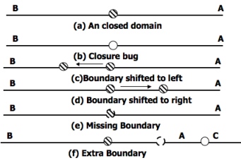
    Figure 4.14: One Dimensional Domain Bugs, Closed Boundaries.

• TESTING TWO DIMENSIONAL DOMAINS:
  • Figure 4.15 shows possible domain boundary bugs for a two-dimensional domain.
  • A and B are adjacent domains and the boundary is closed with respect to A, which means that it is open with respect to B.
    
    
    
    

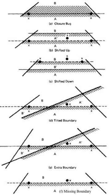
    Figure 4.15: Two Dimensional Domain Bugs.

  • For Closed Boundaries:
    1. Closure Bug: Figure 4.15a shows a faulty closure, such as might be caused by using a wrong operator (for example, x >= k when x > k was intended, or vice versa). The two on points detect this bug because those values will get B rather than A processing.
    2. Shifted Boundary: In Figure 4.15b the bug is a shift up, which converts part of domain B into A processing, denoted by A'. This result is caused by an incorrect constant in a predicate, such as x + y >= 17 when x + y >= 7 was intended. The off point (closed off outside) catches this bug. Figure 4.15c shows a shift down that is caught by the two on points.
    3. Tilted Boundary: A tilted boundary occurs when coefficients in the boundary inequality are wrong. For example, 3x + 7y > 17 when 7x + 3y > 17 was intended. Figure 4.15d has a tilted boundary, which creates erroneous domain segments A' and B'. In this example the bug is caught by the left on point.
    4. Extra Boundary: An extra boundary is created by an extra predicate. An extra boundary will slice through many different domains and will therefore cause many test failures for the same bug. The extra boundary in Figure 4.15e is caught by two on points, and depending on which way the extra boundary goes, possibly by the off point also.
    5. Missing Boundary: A missing boundary is created by leaving a boundary predicate out. A missing boundary will merge different domains and will cause many test failures although there is only one bug. A missing boundary, shown in Figure 4.15f, is caught by the two on points because the processing for A and B is the same - either A or B processing.
• PROCEDURE FOR TESTING: The procedure is conceptually is straight forward. It can be done by hand for two dimensions and for a few domains and practically impossible for more than two variables.
  1. Identify input variables.
  2. Identify variable which appear in domain defining predicates, such as control flow predicates.
  3. Interpret all domain predicates in terms of input variables.
  4. For p binary predicates, there are at most 2^p combinations of TRUE-FALSE values and therefore, at most 2^p domains. Find the set of all non null domains. The result is a boolean expression in the predicates consisting a set of AND terms joined by OR's. For example ABC+DEF+GHI ...... Where the capital letters denote predicates. Each product term is a set of linear inequality that defines a domain or a part of a multiply connected domains.
  5. Solve these inequalities to find all the extreme points of each domain using any of the linear programming methods.

---

DOMAIN AND INTERFACE TESTING

---

• INTRODUCTION:
  • Recall that we defined integration testing as testing the correctness of the interface between two otherwise correct components.
  • Components A and B have been demonstrated to satisfy their component tests, and as part of the act of integrating them we want to investigate possible inconsistencies across their interface.
  • Interface between any two components is considered as a subroutine call.
  • We're looking for bugs in that "call" when we do interface testing.
  • Let's assume that the call sequence is correct and that there are no type incompatibilities.
  • For a single variable, the domain span is the set of numbers between (and including) the smallest value and the largest value. For every input variable we want (at least): compatible domain spans and compatible closures (Compatible but need not be Equal).
• DOMAINS AND RANGE:
  • The set of output values produced by a function is called the range of the function, in contrast with the domain, which is the set of input values over which the function is defined.
  • For most testing, our aim has been to specify input values and to predict and/or confirm output values that result from those inputs.
  • Interface testing requires that we select the output values of the calling routine i.e. caller's range must be compatible with the called routine's domain.
  • An interface test consists of exploring the correctness of the following mappings:
    

                 caller domain --> caller range		(caller unit test)
                 caller range --> called domain		(integration test)
                 called domain --> called range		(called unit test)
                 

• CLOSURE COMPATIBILITY:
  • Assume that the caller's range and the called domain spans the same numbers - for example, 0 to 17.
  • Figure 4.16 shows the four ways in which the caller's range closure and the called's domain closure can agree.
  • The thick line means closed and the thin line means open. Figure 4.16 shows the four cases consisting of domains that are closed both on top (17) and bottom (0), open top and closed bottom, closed top and open bottom, and open top and bottom.
    
    
    
    

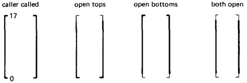
    Figure 4.16: Range / Domain Closure Compatibility.

  • Figure 4.17 shows the twelve different ways the caller and the called can disagree about closure. Not all of them are necessarily bugs. The four cases in which a caller boundary is open and the called is closed (marked with a "?") are probably not buggy. It means that the caller will not supply such values but the called can accept them.
    
    
    
    

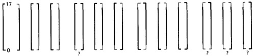
    Figure 4.17: Equal-Span Range / Domain Compatibility Bugs.

• SPAN COMPATIBILITY:
  • Figure 4.18 shows three possibly harmless span incompatibilities.
    
    
    
    

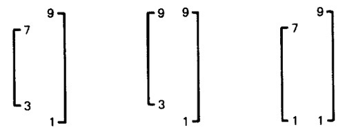
    Figure 4.18: Harmless Range / Domain Span incompatibility bug (Caller Span is smaller than Called).

  • In all cases, the caller's range is a subset of the called's domain. That's not necessarily a bug.
  • The routine is used by many callers; some require values inside a range and some don't. This kind of span incompatibility is a bug only if the caller expects the called routine to validate the called number for the caller.
  • Figure 4.19a shows the opposite situation, in which the called routine's domain has a smaller span than the caller expects. All of these examples are buggy.
    
    
    
    

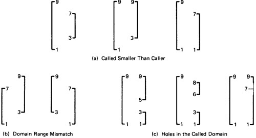
    Figure 4.19: Buggy Range / Domain Mismatches

  • In Figure 4.19b the ranges and domains don't line up; hence good values are rejected, bad values are accepted, and if the called routine isn't robust enough, we have crashes.
  • Figure 4.19c combines these notions to show various ways we can have holes in the domain: these are all probably buggy.
• INTERFACE RANGE / DOMAIN COMPATIBILITY TESTING:
  • For interface testing, bugs are more likely to concern single variables rather than peculiar combinations of two or more variables.
  • Test every input variable independently of other input variables to confirm compatibility of the caller's range and the called routine's domain span and closure of every domain defined for that variable.
  • There are two boundaries to test and it's a one-dimensional domain; therefore, it requires one on and one off point per boundary or a total of two on points and two off points for the domain - pick the off points appropriate to the closure (COOOOI).
  • Start with the called routine's domains and generate test points in accordance to the domain-testing strategy used for that routine in component testing.
  • Unless you're a mathematical whiz you won't be able to do this without tools for more than one variable at a time.

---

DOMAINS AND TESTABILITY

---

To be added

---

SUMMARY:

---

1. Programs can be viewed as doing two different things: (a) classifying input vectors into domains, and (b) doing the processing appropriate to the domain. Domain testing focuses on the classification aspect and explores domain correctness.
2. Domains are specified by the intersections of inequalities obtained by interpreting predicates in terms of input variables. If domain testing is based on structure, the interpretation is specific to the control-flow path through the set of predicates that define the domain. If domain testing is based on specifications, the interpretation is specific to the path through a specification data flowgraph.
3. Every domain boundary has a closure that specifies whether boundary points are or are not in the domain. Closure verification is a big part of domain testing.
4. Almost all domain boundaries found in practice are based on linear inequalities. Those that aren't can often be converted to linear inequalities by a suitable linearization transformation.
5. Nice domains have the following properties: linear boundaries, boundaries that extend from plus to minus infinity in all variables, have systematic inequality sets, form orthogonal sets, have consistent closures, are convex, and create domains that are all in one piece. Nice domains are easy to test because the boundaries can be tested one at a time, independently of the other boundaries. If domains aren't nice, examine the specifications to see whether they can be changed to make the boundaries nice; often what's difficult about a boundary or domain is arbitrary rather than based on real requirements.
6. As designers, guard against incorrect simplifications and transformations that make essentially ugly domains nice. As testers, look for such transformations.
7. The general domain strategy for arbitrary convex, simply connected, linear domains is based on testing at most (n + 1)p test points per domain, where n is the dimension of the interpreted input space and p is the number of boundaries in the domain. Of these, n points are on points and one is an off point. Remember the definition of off point - COOOOI.
8. Real domains, especially if they have nice boundaries, can be tested in far less than (n + 1)p points: as little as O(n).
9. Domain testing is easy for one dimension, difficult for two, and tool-intensive for more than two. Beg, borrow, or build the tools before you attempt to apply domain testing to the general situation. Finding the test points is a linear programming problem for the general case and trivial for the nicest domains.
10. Domain testing is only one of many related partition testing methods which includes more points, such as n-on + n-off, or extreme points and off-extreme points. Extreme points are good because bugs tend to congregate there.
11. The domain-testing outlook is a productive tactic for integration interface testing. Test range/domain compatibility between caller and called routines and all other forms of intercomponent communications.