HOME

SCHEDULE

RESOURCES

GLOSSARY

ASSIGNMENTS

TRANSACTION FLOW TESTING AND DATA FLOW TESTING:

This unit gives an indepth overview of two forms of functional or system testing namely Transaction Flow Testing and Data Flow Testing.

At the end of this unit, the student will be able to:

• Understand the concept of transaction flow testing and data flow testing.
• Visualize the transaction flow and data flow in a software system.
• Understand the need and appreciate the usage of the two testing methods.
• Identify the complications in a transaction flow testing method and anomalies in data flow testing.
• Interpret the data flow anomaly state graphs and control flow grpahs and represent the state of the data objetcs.
• Understand the limitations of Static analysis in data flow testing.
• Compare and analyze various strategies of data flow testing.

---

TRANSACTION FLOWS:

---

• INTRODUCTION:
  • A transaction is a unit of work seen from a system user's point of view.
  • A transaction consists of a sequence of operations, some of which are performed by a system, persons or devices that are outside of the system.
  • Transaction begin with Birth-that is they are created as a result of some external act.
  • At the conclusion of the transaction's processing, the transaction is no longer in the system.
  • Example of a transaction: A transaction for an online information retrieval system might consist of the following steps or tasks:
    
    • Accept input (tentative birth)
    • Validate input (birth)
    • Transmit acknowledgement to requester
    • Do input processing
    • Search file
    • Request directions from user
    • Accept input
    • Validate input
    • Process request
    • Update file
    • Transmit output
    • Record transaction in log and clean up (death)
• TRANSACTION FLOW GRAPHS:
  • Transaction flows are introduced as a representation of a system's processing.
  • The methods that were applied to control flow graphs are then used for functional testing.
  • Transaction flows and transaction flow testing are to the independent system tester what control flows are path testing are to the programmer.
  • The transaction flow graph is to create a behavioral model of the program that leads to functional testing.
  • The transaction flowgraph is a model of the structure of the system's behavior (functionality).
  • An example of a Transaction Flow is as follows:
    
    
    
    

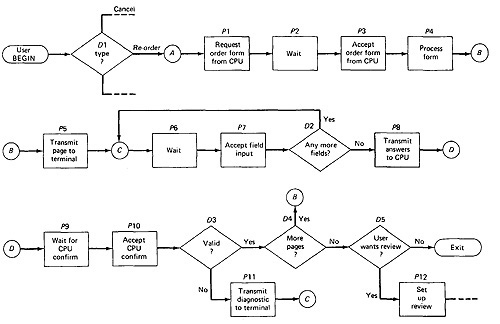
    Figure 3.1: An Example of a Transaction Flow

• USAGE:
  • Transaction flows are indispensable for specifying requirements of complicated systems, especially online systems.
  • A big system such as an air traffic control or airline reservation system, has not hundreds, but thousands of different transaction flows.
  • The flows are represented by relatively simple flowgraphs, many of which have a single straight-through path.
  • Loops are infrequent compared to control flowgraphs.
  • The most common loop is used to request a retry after user input errors. An ATM system, for example, allows the user to try, say three times, and will take the card away the fourth time.
• COMPLICATIONS:
  • In simple cases, the transactions have a unique identity from the time they're created to the time they're completed.
  • In many systems the transactions can give birth to others, and transactions can also merge.
  • Births:There are three different possible interpretations of the decision symbol, or nodes with two or more out links. It can be a Decision, Biosis or a Mitosis.
    1. Decision:Here the transaction will take one alternative or the other alternative but not both. (See Figure 3.2 (a))
    2. Biosis:Here the incoming transaction gives birth to a new transaction, and both transaction continue on their separate paths, and the parent retains it identity. (See Figure 3.2 (b))
    3. Mitosis:Here the parent transaction is destroyed and two new transactions are created.(See Figure 3.2 (c))
    
    
    
    
    

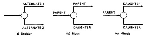
    Figure 3.2: Nodes with multiple outlinks

  • Mergers:Transaction flow junction points are potentially as troublesome as transaction flow splits. There are three types of junctions: (1) Ordinary Junction (2) Absorption (3) Conjugation
    1. Ordinary Junction: An ordinary junction which is similar to the junction in a control flow graph. A transaction can arrive either on one link or the other. (See Figure 3.3 (a))
    2. Absorption: In absorption case, the predator transaction absorbs prey transaction. The prey gone but the predator retains its identity. (See Figure 3.3 (b))
    3. Conjugation: In conjugation case, the two parent transactions merge to form a new daughter. In keeping with the biological flavor this case is called as conjugation.(See Figure 3.3 (c))
    
    
    
    
    

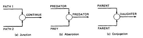
    Figure 3.3: Transaction Flow Junctions and Mergers

  • We have no problem with ordinary decisions and junctions. Births, absorptions, and conjugations are as problematic for the software designer as they are for the software modeler and the test designer; as a consequence, such points have more than their share of bugs. The common problems are: lost daughters, wrongful deaths, and illegitimate births.

---

TRANSACTION FLOW TESTING TECHNIQUES:

---

• GET THE TRANSACTIONS FLOWS:
  • Complicated systems that process a lot of different, complicated transactions should have explicit representations of the transactions flows, or the equivalent.
  • Transaction flows are like control flow graphs, and consequently we should expect to have them in increasing levels of detail.
  • The system's design documentation should contain an overview section that details the main transaction flows.
  • Detailed transaction flows are a mandatory pre requisite to the rational design of a system's functional test.
• INSPECTIONS, REVIEWS AND WALKTHROUGHS:
  • Transaction flows are natural agenda for system reviews or inspections.
  • In conducting the walkthroughs, you should:
    • Discuss enough transaction types to account for 98%-99% of the transaction the system is expected to process.
    • Discuss paths through flows in functional rather than technical terms.
    • Ask the designers to relate every flow to the specification and to show how that transaction, directly or indirectly, follows from the requirements.
  • Make transaction flow testing the corner stone of system functional testing just as path testing is the corner stone of unit testing.
  • Select additional flow paths for loops, extreme values, and domain boundaries.
  • Design more test cases to validate all births and deaths.
  • Publish and distribute the selected test paths through the transaction flows as early as possible so that they will exert the maximum beneficial effect on the project.
• PATH SELECTION:
  • Select a set of covering paths (c1+c2) using the analogous criteria you used for structural path testing.
  • Select a covering set of paths based on functionally sensible transactions as you would for control flow graphs.
  • Try to find the most tortuous, longest, strangest path from the entry to the exit of the transaction flow.
• PATH SENSITIZATION:
  • Most of the normal paths are very easy to sensitize-80% - 95% transaction flow coverage (c1+c2) is usually easy to achieve.
  • The remaining small percentage is often very difficult.
  • Sensitization is the act of defining the transaction. If there are sensitization problems on the easy paths, then bet on either a bug in transaction flows or a design bug.
• PATH INSTRUMENTATION:
  • Instrumentation plays a bigger role in transaction flow testing than in unit path testing.
  • The information of the path taken for a given transaction must be kept with that transaction and can be recorded by a central transaction dispatcher or by the individual processing modules.
  • In some systems, such traces are provided by the operating systems or a running log.

---

IMPLEMENTATION:

---

To be added

---

BASICS OF DATA FLOW TESTING:

---

• DATA FLOW TESTING:
  • Data flow testing is the name given to a family of test strategies based on selecting paths through the program's control flow in order to explore sequences of events related to the status of data objects.
  • For example, pick enough paths to assure that every data object has been initialized prior to use or that all defined objects have been used for something.
  • Motivation:

    it is our belief that, just as one would not feel confident about a program without executing every statement in it as part of some test, one should not feel confident about a program without having seen the effect of using the value produced by each and every computation.

• DATA FLOW MACHINES:
  • There are two types of data flow machines with different architectures. (1) Von Neumann machnes (2) Multi-instruction, multi-data machines (MIMD).
  • Von Neumann Machine Architecture:
    • Most computers today are von-neumann machines.
    • This architecture features interchangeable storage of instructions and data in the same memory units.
    • The Von Neumann machine Architecture executes one instruction at a time in the following, micro instruction sequence:
      1. Fetch instruction from memory
      2. Interpret instruction
      3. Fetch operands
      4. Process or Execute
      5. Store result
      6. Increment program counter
      7. GOTO 1
  • Multi-instruction, Multi-data machines (MIMD) Architecture:
    • These machines can fetch several instructions and objects in parallel.
    • They can also do arithmetic and logical operations simultaneously on different data objects.
    • The decision of how to sequence them depends on the compiler.
• BUG ASSUMPTION:
  • The bug assumption for data-flow testing strategies is that control flow is generally correct and that something has gone wrong with the software so that data objects are not available when they should be, or silly things are being done to data objects.
  • Also, if there is a control-flow problem, we expect it to have symptoms that can be detected by data-flow analysis.
  • Although we'll be doing data-flow testing, we won't be using data flowgraphs as such. Rather, we'll use an ordinary control flowgraph annotated to show what happens to the data objects of interest at the moment.
• DATA FLOW GRAPHS:
  • The data flow graph is a graph consisting of nodes and directed links.
    
    
    
    

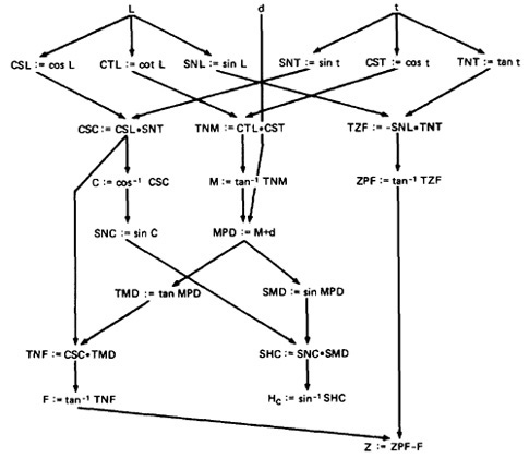
    Figure 3.4: Example of a data flow graph

  • We will use an control graph to show what happens to data objects of interest at that moment.
  • Our objective is to expose deviations between the data flows we have and the data flows we want.
  • Data Object State and Usage:
    • Data Objects can be created, killed and used.
    • They can be used in two distinct ways: (1) In a Calculation (2) As a part of a Control Flow Predicate.
    • The following symbols denote these possibilities:
      1. Defined: d - defined, created, initialized etc
      2. Killed or undefined: k - killed, undefined, released etc
      3. Usage: u - used for something (c - used in Calculations, p - used in a predicate)
    • 1. Defined (d):
      • An object is defined explicitly when it appears in a data declaration.
      • Or implicitly when it appears on the left hand side of the assignment.
      • It is also to be used to mean that a file has been opened.
      • A dynamically allocated object has been allocated.
      • Something is pushed on to the stack.
      • A record written.
    • 2. Killed or Undefined (k):
      • An object is killed on undefined when it is released or otherwise made unavailable.
      • When its contents are no longer known with certitude (with aboslute certainity / perfectness).
      • Release of dynamically allocated objects back to the availability pool.
      • Return of records.
      • The old top of the stack after it is popped.
      • An assignment statement can kill and redefine immediately. For example, if A had been previously defined and we do a new assignment such as A : = 17, we have killed A's previous value and redefined A
    • 3. Usage (u):
      • A variable is used for computation (c) when it appears on the right hand side of an assignment statement.
      • A file record is read or written.
      • It is used in a Predicate (p) when it appears directly in a predicate.
• DATA FLOW ANOMALIES:
  • An anomaly is denoted by a two-character sequence of actions.
  • For example, ku means that the object is killed and then used, where as dd means that the object is defined twice without an intervening usage.
  • What is an anomaly is depend on the application.
  • There are nine possible two-letter combinations for d, k and u. some are bugs, some are suspicious, and some are okay.
    1. dd :- probably harmless but suspicious. Why define the object twice without an intervening usage?
    2. dk :- probably a bug. Why define the object without using it?
    3. du :- the normal case. The object is defined and then used.
    4. kd :- normal situation. An object is killed and then redefined.
    5. kk :- harmless but probably buggy. Did you want to be sure it was really killed?
    6. ku :- a bug. the object doesnot exist.
    7. ud :- usually not a bug because the language permits reassignment at almost any time.
    8. uk :- normal situation.
    9. uu :- normal situation.
  • In addition to the two letter situations, there are six single letter situations.
  • We will use a leading dash to mean that nothing of interest (d,k,u) occurs prior to the action noted along the entry-exit path of interest.
  • A trailing dash to mean that nothing happens after the point of interest to the exit.
  • They possible anomalies are:
    1. -k :- possibly anomalous because from the entrance to this point on the path, the variable had not been defined. We are killing a variable that does not exist.
    2. -d :- okay. This is just the first definition along this path.
    3. -u :- possibly anomalous. Not anomalous if the variable is global and has been previously defined.
    4. k- :- not anomalous. The last thing done on this path was to kill the variable.
    5. d- :- possibly anomalous. The variable was defined and not used on this path. But this could be a global definition.
    6. u- :- not anomalous. The variable was used but not killed on this path. Although this sequence is not anomalous, it signals a frequent kind of bug. If d and k mean dynamic storage allocation and return respectively, this could be an instance in which a dynamically allocated object was not returned to the pool after use.
• DATA FLOW ANOMALY STATE GRAPH:
  • Data flow anomaly model prescribes that an object can be in one of four distinct states:
    1. K :- undefined, previously killed, doesnot exist
    2. D :- defined but not yet used for anything
    3. U :- has been used for computation or in predicate
    4. A :- anomalous
  • These capital letters (K,D,U,A) denote the state of the variable and should not be confused with the program action, denoted by lower case letters.
  • Unforgiving Data - Flow Anomaly Flow Graph:Unforgiving model, in which once a variable becomes anomalous it can never return to a state of grace.
    
    
    
    

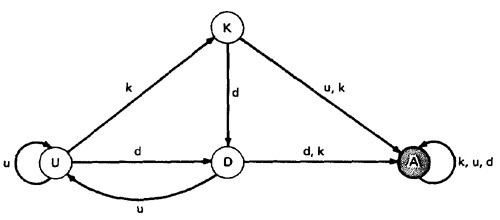
    Figure 3.5: Unforgiving Data Flow Anomaly State Graph

    Assume that the variable starts in the K state - that is, it has not been defined or does not exist. If an attempt is made to use it or to kill it (e.g., say that we're talking about opening, closing, and using files and that 'killing' means closing), the object's state becomes anomalous (state A) and, once it is anomalous, no action can return the variable to a working state. If it is defined (d), it goes into the D, or defined but not yet used, state. If it has been defined (D) and redefined (d) or killed without use (k), it becomes anomalous, while usage (u) brings it to the U state. If in U, redefinition (d) brings it to D, u keeps it in U, and k kills it.
  • Forgiving Data - Flow Anomaly Flow Graph:Forgiving model is an alternate model where redemption (recover) from the anomalous state is possible.
    
    
    
    

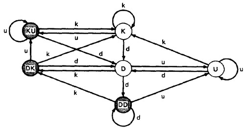
    Figure 3.6: Forgiving Data Flow Anomaly State Graph

    This graph has three normal and three anomalous states and he considers the kk sequence not to be anomalous. The difference between this state graph and Figure 3.5 is that redemption is possible. A proper action from any of the three anomalous states returns the variable to a useful working state.
    
    The point of showing you this alternative anomaly state graph is to demonstrate that the specifics of an anomaly depends on such things as language, application, context, or even your frame of mind. In principle, you must create a new definition of data flow anomaly (e.g., a new state graph) in each situation. You must at least verify that the anomaly definition behind the theory or imbedded in a data flow anomaly test tool is appropriate to your situation.
• STATIC Vs DYNAMIC ANOMALY DETECTION:
  • Static analysis is analysis done on source code without actually executing it. For example: source code syntax error detection is the static analysis result.
  • Dynamic analysis is done on the fly as the program is being executed and is based on intermediate values that result from the program's execution. For example: a division by zero warning is the dynamic result.
  • If a problem, such as a data flow anomaly, can be detected by static analysis methods, then it doesnot belongs in testing - it belongs in the language processor.
  • There is actually a lot more static analysis for data flow analysis for data flow anomalies going on in current language processors.
  • For example, language processors which force variable declarations can detect (-u) and (ku) anomalies.
  • But still there are many things for which current notions of static analysis are INADEQUATE.
  • Why Static Analysis isn't enough? There are many things for which current notions of static analysis are inadequate. They are:
    • Dead Variables:Although it is often possible to prove that a variable is dead or alive at a given point in the program, the general problem is unsolvable.
    • Arrays:Arrays are problematic in that the array is defined or killed as a single object, but reference is to specific locations within the array. Array pointers are usually dynamically calculated, so there's no way to do a static analysis to validate the pointer value. In many languages, dynamically allocated arrays contain garbage unless explicitly initialized and therefore, -u anomalies are possible.
    • Records and Pointers:The array problem and the difficulty with pointers is a special case of multipart data structures. We have the same problem with records and the pointers to them. Also, in many applications we create files and their names dynamically and there's no way to determine, without execution, whether such objects are in the proper state on a given path or, for that matter, whether they exist at all.
    • Dynamic Subroutine and Function Names in a Call:subroutine or function name is a dynamic variable in a call. What is passed, or a combination of subroutine names and data objects, is constructed on a specific path. There's no way, without executing the path, to determine whether the call is correct or not.
    • False Anomalies:Anomalies are specific to paths. Even a "clear bug" such as ku may not be a bug if the path along which the anomaly exist is unachievable. Such "anomalies" are false anomalies. Unfortunately, the problem of determining whether a path is or is not achievable is unsolvable.
    • Recoverable Anomalies and Alternate State Graphs:What constitutes an anomaly depends on context, application, and semantics. How does the compiler know which model I have in mind? It can't because the definition of "anomaly" is not fundamental. The language processor must have a built-in anomaly definition with which you may or may not (with good reason) agree.
    • Concurrency, Interrupts, System Issues:As soon as we get away from the simple single-task uniprocessor environment and start thinking in terms of systems, most anomaly issues become vastly more complicated. How often do we define or create data objects at an interrupt level so that they can be processed by a lower-priority routine? Interrupts can make the "correct" anomalous and the "anomalous" correct. True concurrency (as in an MIMD machine) and pseudoconcurrency (as in multiprocessing) systems can do the same to us. Much of integration and system testing is aimed at detecting data-flow anomalies that cannot be detected in the context of a single routine.
  • Although static analysis methods have limits, they are worth using and a continuing trend in language processor design has been better static analysis methods, especially for data flow anomaly detection. That's good because it means there's less for us to do as testers and we have far too much to do as it is.
• DATA FLOW MODEL:
  • The data flow model is based on the program's control flow graph - Don't confuse that with the program's data flowgraph..
  • Here we annotate each link with symbols (for example, d, k, u, c, p) or sequences of symbols (for example, dd, du, ddd) that denote the sequence of data operations on that link with respect to the variable of interest. Such annotations are called link weights.
  • The control flow graph structure is same for every variable: it is the weights that change.
  • Components of the model:
    1. To every statement there is a node, whose name is unique. Every node has at least one outlink and at least one inlink except for exit nodes and entry nodes.
    2. Exit nodes are dummy nodes placed at the outgoing arrowheads of exit statements (e.g., END, RETURN), to complete the graph. Similarly, entry nodes are dummy nodes placed at entry statements (e.g., BEGIN) for the same reason.
    3. The outlink of simple statements (statements with only one outlink) are weighted by the proper sequence of data-flow actions for that statement. Note that the sequence can consist of more than one letter. For example, the assignment statement A:= A + B in most languages is weighted by cd or possibly ckd for variable A. Languages that permit multiple simultaneous assignments and/or compound statements can have anomalies within the statement. The sequence must correspond to the order in which the object code will be executed for that variable.
    4. Predicate nodes (e.g., IF-THEN-ELSE, DO WHILE, CASE) are weighted with the p - use(s) on every outlink, appropriate to that outlink.
    5. Every sequence of simple statements (e.g., a sequence of nodes with one inlink and one outlink) can be replaced by a pair of nodes that has, as weights on the link between them, the concatenation of link weights.
    6. If there are several data-flow actions on a given link for a given variable, then the weight of the link is denoted by the sequence of actions on that link for that variable.
    7. Conversely, a link with several data-flow actions on it can be replaced by a succession of equivalent links, each of which has at most one data-flow action for any variable.
  • Let us consider the example:
    
    
    
    

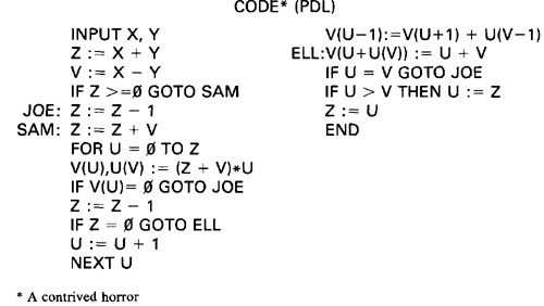
    Figure 3.7: Program Example (PDL)

    ---

    
    
    
    
    

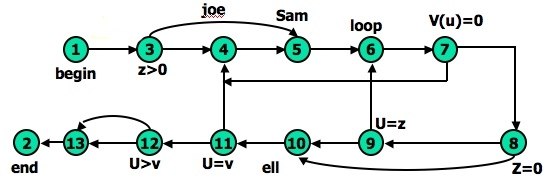
    Figure 3.8: Unannotated flowgraph for example program in Figure 3.7

    ---

    
    
    
    
    

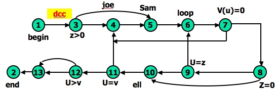
    Figure 3.9: Control flowgraph annotated for X and Y data flows.

    ---

    
    
    
    
    

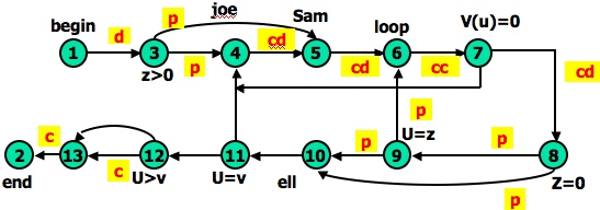
    Figure 3.10: Control flowgraph annotated for Z data flow.

    ---

    
    
    
    
    

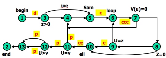
    Figure 3.11: Control flowgraph annotated for V data flow.

    ---

---

STRATEGIES OF DATA FLOW TESTING:

---

• INTRODUCTION:
  • Data Flow Testing Strategies are structural strategies.
  • In contrast to the path-testing strategies, data-flow strategies take into account what happens to data objects on the links in addition to the raw connectivity of the graph.
  • In other words, data flow strategies require data-flow link weights (d,k,u,c,p).
  • Data Flow Testing Strategies are based on selecting test path segments (also called sub paths) that satisfy some characteristic of data flows for all data objects.
  • For example, all subpaths that contain a d (or u, k, du, dk).
  • A strategy X is stronger than another strategy Y if all test cases produced under Y are included in those produced under X - conversely for weaker.
• TERMINOLOGY:
  1. Definition-Clear Path Segment, with respect to variable X, is a connected sequence of links such that X is (possibly) defined on the first link and not redefined or killed on any subsequent link of that path segment. ll paths in Figure 3.9 are definition clear because variables X and Y are defined only on the first link (1,3) and not thereafter. In Figure 3.10, we have a more complicated situation. The following path segments are definition-clear: (1,3,4), (1,3,5), (5,6,7,4), (7,8,9,6,7), (7,8,9,10), (7,8,10), (7,8,10,11). Subpath (1,3,4,5) is not definition-clear because the variable is defined on (1,3) and again on (4,5). For practice, try finding all the definition-clear subpaths for this routine (i.e., for all variables).
  2. Loop-Free Path Segment is a path segment for which every node in it is visited atmost once. For Example, path (4,5,6,7,8,10) in Figure 3.10 is loop free, but path (10,11,4,5,6,7,8,10,11,12) is not because nodes 10 and 11 are each visited twice.
  3. Simple path segment is a path segment in which at most one node is visited twice. For example, in Figure 3.10, (7,4,5,6,7) is a simple path segment. A simple path segment is either loop-free or if there is a loop, only one node is involved.
  4. A du path from node i to k is a path segment such that if the last link has a computational use of X, then the path is simple and definition-clear; if the penultimate (last but one) node is j - that is, the path is (i,p,q,...,r,s,t,j,k) and link (j,k) has a predicate use - then the path from i to j is both loop-free and definition-clear.
• STRATEGIES: The structural test strategies discussed below are based on the program's control flowgraph. They differ in the extent to which predicate uses and/or computational uses of variables are included in the test set. Various types of data flow testing strategies in decreasing order of their effectiveness are:
  
  
  1. All - du Paths (ADUP): The all-du-paths (ADUP) strategy is the strongest data-flow testing strategy discussed here. It requires that every du path from every definition of every variable to every use of that definition be exercised under some test.
     
     For variable X and Y:In Figure 3.9, because variables X and Y are used only on link (1,3), any test that starts at the entry satisfies this criterion (for variables X and Y, but not for all variables as required by the strategy).
     
     For variable Z: The situation for variable Z (Figure 3.10) is more complicated because the variable is redefined in many places. For the definition on link (1,3) we must exercise paths that include subpaths (1,3,4) and (1,3,5). The definition on link (4,5) is covered by any path that includes (5,6), such as subpath (1,3,4,5,6, ...). The (5,6) definition requires paths that include subpaths (5,6,7,4) and (5,6,7,8).
     
     For variable V: Variable V (Figure 3.11) is defined only once on link (1,3). Because V has a predicate use at node 12 and the subsequent path to the end must be forced for both directions at node 12, the all-du-paths strategy for this variable requires that we exercise all loop-free entry/exit paths and at least one path that includes the loop caused by (11,4). Note that we must test paths that include both subpaths (3,4,5) and (3,5) even though neither of these has V definitions. They must be included because they provide alternate du paths to the V use on link (5,6). Although (7,4) is not used in the test set for variable V, it will be included in the test set that covers the predicate uses of array variable V() and U.
     
     The all-du-paths strategy is a strong criterion, but it does not take as many tests as it might seem at first because any one test simultaneously satisfies the criterion for several definitions and uses of several different variables.
     
     
  2. All Uses Startegy (AU):The all uses strategy is that at least one definition clear path from every definition of every variable to every use of that definition be exercised under some test. Just as we reduced our ambitions by stepping down from all paths (P) to branch coverage (C2), say, we can reduce the number of test cases by asking that the test set should include at least one path segment from every definition to every use that can be reached by that definition.
     
     For variable V: In Figure 3.11, ADUP requires that we include subpaths (3,4,5) and (3,5) in some test because subsequent uses of V, such as on link (5,6), can be reached by either alternative. In AU either (3,4,5) or (3,5) can be used to start paths, but we don't have to use both. Similarly, we can skip the (8,10) link if we've included the (8,9,10) subpath. Note the hole. We must include (8,9,10) in some test cases because that's the only way to reach the c use at link (9,10) - but suppose our bug for variable V is on link (8,10) after all? Find a covering set of paths under AU for Figure 3.11.
     
     
  3. All p-uses/some c-uses strategy (APU+C) : For every variable and every definition of that variable, include at least one definition free path from the definition to every predicate use; if there are definitions of the variables that are not covered by the above prescription, then add computational use test cases as required to cover every definition.
     
     For variable Z:In Figure 3.10, for APU+C we can select paths that all take the upper link (12,13) and therefore we do not cover the c-use of Z: but that's okay according to the strategy's definition because every definition is covered. Links (1,3), (4,5), (5,6), and (7,8) must be included because they contain definitions for variable Z. Links (3,4), (3,5), (8,9), (8,10), (9,6), and (9,10) must be included because they contain predicate uses of Z. Find a covering set of test cases under APU+C for all variables in this example - it only takes two tests.
     
     For variable V:In Figure 3.11, APU+C is achieved for V by (1,3,5,6,7,8,10,11,4,5,6,7,8,10,11,12[upper], 13,2) and (1,3,5,6,7,8,10,11,12[lower], 13,2). Note that the c-use at (9,10) need not be included under the APU+C criterion.
     
     
  4. All c-uses/some p-uses strategy (ACU+P) : The all c-uses/some p-uses strategy (ACU+P) is to first ensure coverage by computational use cases and if any definition is not covered by the previously selected paths, add such predicate use cases as are needed to assure that every definition is included in some test.
     
     For variable Z: In Figure 3.10, ACU+P coverage is achieved for Z by path (1,3,4,5,6,7,8,10, 11,12,13[lower], 2), but the predicate uses of several definitions are not covered. Specifically, the (1,3) definition is not covered for the (3,5) p-use, the (7,8) definition is not covered for the (8,9), (9,6) and (9, 10) p-uses.
     
     

     The above examples imply that APU+C is stronger than branch coverage but ACU+P may be weaker than, or incomparable to, branch coverage.

  5. All Definitions Strategy (AD) : The all definitions strategy asks only every definition of every variable be covered by atleast one use of that variable, be that use a computational use or a predicate use.
     
     For variable Z: Path (1,3,4,5,6,7,8, . . .) satisfies this criterion for variable Z, whereas any entry/exit path satisfies it for variable V.
     
     

     From the definition of this strategy we would expect it to be weaker than both ACU+P and APU+C.

  6. All Predicate Uses (APU), All Computational Uses (ACU) Strategies : The all predicate uses strategy is derived from APU+C strategy by dropping the requirement that we include a c-use for the variable if there are no p-uses for the variable. The all computational uses strategy is derived from ACU+P strategy by dropping the requirement that we include a p-use for the variable if there are no c-uses for the variable.
     
     

     It is intuitively obvious that ACU should be weaker than ACU+P and that APU should be weaker than APU+C.

• ORDERING THE STRATEGIES:
  • Figure 3.12 compares path-flow and data-flow testing strategies. The arrows denote that the strategy at the arrow's tail is stronger than the strategy at the arrow's head.
    
    
    
    

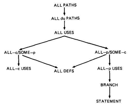
    Figure 3.12: Relative Strength of Structural Test Strategies.

  • The right-hand side of this graph, along the path from "all paths" to "all statements" is the more interesting hierarchy for practical applications.
  • Note that although ACU+P is stronger than ACU, both are incomparable to the predicate-biased strategies. Note also that "all definitions" is not comparable to ACU or APU.
• SLICING AND DICING:
  • A (static) program slice is a part of a program (e.g., a selected set of statements) defined with respect to a given variable X (where X is a simple variable or a data vector) and a statement i: it is the set of all statements that could (potentially, under static analysis) affect the value of X at statement i - where the influence of a faulty statement could result from an improper computational use or predicate use of some other variables at prior statements.
  • If X is incorrect at statement i, it follows that the bug must be in the program slice for X with respect to i
  • A program dice is a part of a slice in which all statements which are known to be correct have been removed.
  • In other words, a dice is obtained from a slice by incorporating information obtained through testing or experiment (e.g., debugging).
  • The debugger first limits her scope to those prior statements that could have caused the faulty value at statement i (the slice) and then eliminates from further consideration those statements that testing has shown to be correct.
  • Debugging can be modeled as an iterative procedure in which slices are further refined by dicing, where the dicing information is obtained from ad hoc tests aimed primarily at eliminating possibilities. Debugging ends when the dice has been reduced to the one faulty statement.
  • Dynamic slicing is a refinement of static slicing in which only statements on achievable paths to the statement in question are included.

---

APPLICATION OF DATA FLOW TESTING:

---

To be added

---

SUMMARY:

---

• The methods discussed for path testing of units and programs can be applied with suitable interpretation to functional testing based on transaction flows.
• The biggest problem and the biggest payoff may be getting the transaction flows in the first place.
• Full coverage (C1 + C2) is required for all flows, but most bugs will be found on the strange, meaningless, weird paths.
• Transaction-flow control may be implemented by means of an undeclared and unrecognized internal language.
• The practice of attempting to design tests based on transaction-flow representation of requirements and discussing those attempts with the designer can unearth more bugs than any tests you run.
• Data are as important as code and will become more important.
• Data integrity is as important as code integrity. Just as common sense dictates that all statements and branches be exercised on under test, all data definitions and subsequent uses must similarly be tested.
• What constitutes a data flow anomaly is peculiar to the application. Be sure to have a clear concept of data flow anomalies in your situation.
• Use all available tools to detect those anomalies that can be detected statically. Let the extent and excellence of static data-flow anomaly detection be as important a criterion in selecting a language processor as produced object code efficiency and compilation speed. Use the slower compiler that gives you slower object code if it can detect more anomalies. You can always recompile the unit after it has been debugged.
• The data-flow testing strategies span the gap between all paths and branch testing. Of the various available strategies, AU probably has the best payoff for the money. It seems to be no worse than twice the number of test cases required for branch testing, but the resulting code is much more reliable. AU is not too difficult to do without supporting tools, but use the tools as they become available.
• Don't restrict your notion of data-flow anomaly to the obvious. The symbols d, k, u, and the associated anomalies, can be interpreted (with profit) in terms of file opening and closing, resource management, and other applications.